We will learn how to calculate the Average mean, mode, and standard deviation in Google Sheets in this tutorial. We will learn how to use Google Sheets’ statistics measures. There are numerous formulae and metrics available in statistics that can be used to tackle challenging probability, statistics, and math problems. The average, mean, and standard deviation are the most prevalent fundamental ideas that probably spring to mind. These and a lot more will be taught to us today. You can now rejoice because we will be entering the statistical formulas in the series of tutorials on Google Sheets.
Average, mean, mode and standard deviation
Most of us have taken math classes where we studied probability and statistics, or perhaps we studied them separately. Whether we like it or not, most of us had to study it as adults, so you should be excited about it, right? If not, I’m here to add some excitement to the learning process. Everyone is naturally curious about math, especially probability and statistics because they work with real data and provide examples from real-world situations. Fortunately, modern software products like Google Sheets are trained to recognize mathematical formulas and can assist us in applying them to real-world data that is stored on Google Sheets. Thus, we must learn how to use Google Sheets to compute the average mean and standard deviation.
How to Calculate Average, Mean, Mode and Standard Deviation in Google Sheets
I would love to guide you guys toward putting these formulas into practice, as we have already covered the subject in the introductory portions above. As is customary, this article will be divided into numerous sections, each of which will focus on a distinct aspect of the subject. We’ll see illustrations and a step-by-step breakdown of how to address a specific issue.
From the primary topic of how to compute the average mean and standard deviation in Google Sheets, we will see how to calculate the average in the first section.
You may also like>>> How To Slice A String In Google Sheets [4 Ways]
How to calculate Average in Google Sheets
First, let’s define what average is. The middle number in a set of data is called the average. Stated differently, the calculation involves summing up all the numbers and dividing the result by the total number of numbers. We refer to it as Average. Assume I have the following set of data: 1, 2, 3, 4, 5. What will the mean be? Assuming that all of the numbers in the range are added up to 15, the average of the range may be found by dividing the total number of numbers (5) by the sum of the numbers (15). This yields a formula of 15/5 and a result of 3. This is the operation of a simple average function. However, Google Sheets has a straightforward formula =Average(range) that computes the average for us automatically. We’ll explore its application.
Step 1>
Provide a sample data range.

Step 2>
In any other cell, enter the formula =average.

Step 3>
Use the formula to pass your range.

Step 4>
Once you press Enter, the average figure shows.


However, what if some of the values in your data are zeros and you don’t want zeros in the formula? For you, there is a trick.
How to calculate Average excluding zeroes in Google Sheets
There are two ways to compute an average: one with zeroes and one without. Since zeroes can have a significant impact on the average result, we sometimes want to exclude them. In this section, we’ll look at how to calculate an average without zeros. We have a variant of the =Average formula for this, called =AverageIF(). To ignore the zeroes in the specified range, we will use =AverageIF() and pass the condition.
In this example, I’ll use a data range and calculate the average of two adjacent cells—one with zeros and the other without—for that range.
Step 1>
Select a data range that contains one or more zeros.

Step 2>
Determine the range’s average for a chosen cell.


Step 3>
Write the formula =AverageIF() into a different cell.

Step 4>
Provide the parameters in the =AverageIF formula.

Step 5>
For the =AverageIF formula, pass the if condition.

Step 6>
Press Enter to view the difference between the two average numbers.
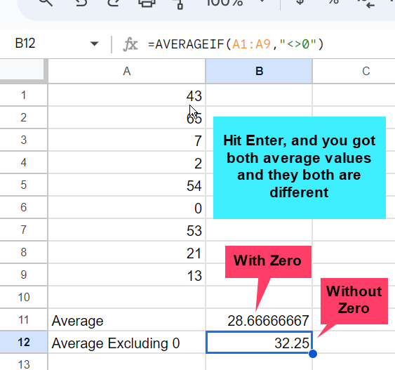
The formula used in this section
=averageif(“<>0,”A1:A9”)
You’ve seen how to determine two separate average values—one with zeros and the other without.

However, I believe there are still some questions. Let me clarify. Often, we have certain hidden data for certain uncommon circumstances. However, the hidden values are automatically included in the average calculation; therefore, how can we ignore or omit the hidden values in our average formula? We shall witness the identical issue in the section below.
How to calculate Average neglecting hidden rows in Google Sheets
This section will explain how to calculate the average in Google Sheets while ignoring hidden rows. By default, if you try to calculate the average of a range that contains some hidden rows with values, the =average formula will include the hidden values as well. However, you can choose to exclude the hidden values from the calculation by hiding them. Another use case is when you want to calculate the average but there are some values in your range that are too high or too low that you want to ignore. In this case, you hide the values and then calculate the average, but nothing will change—the =average formula will include them. Thus, there is a fix, and we will discuss it in this part.
I can provide a sample dummy data range to demonstrate how to use this technique. I have several nearing and common values in this data, but one value is very varied in terms of its value. To prevent my average value from changing drastically as a result of using such a high average, I shall conceal the figure. This is simply an example of a use case; there could be a variety of reasons to exclude or disregard one or more numbers when using Google Sheets to calculate the average.
Step 1>
Bring a few sample data sets.

Step 2>
Remove any rows from your range that you don’t wish to include in the data.
to hide choose the rows, then right-click to hide rows

Step 3>
Let’s attempt to use the normal average.

Step 4>
Let’s now reveal the rows and use the same method to attempt again.

Step 5>
Now, hide rows once more, and enter the =subtotal formula.

Step 6>
Proceed with the initial default argument (101)

Step 7>
Pass the data range, being careful to hide any undesirable data.

Step 8>
Press Enter to finish.

Step 9>
Now that the hidden rows have been revealed, you can verify by seeing a change in the average value.

The equation applied in this section
=SUBTOTAL (101,A1:A9)
This is how easily you can use a subtotal formula to get the average value and hide some of the numbers to exclude them.
Overall, this was a thorough segment; let’s go on to the next one.
How to find or calculate Mean or Median in Google Sheets
This part will teach you how to get the median in Google Sheets. This is a really simple process, so let’s speak about it first. What does the median stand for? There are several differences, despite the common belief that it is the same as average.
The average is calculated by dividing the total number by the sum of the numbers.
The center value, or median, is the point at which half of the observations are larger and half are smaller.
I’m sure it crossed your mind. Below is an example to help you understand the differences between them. To examine the variations, we are going to calculate the average and median for the identical set of data.
I have a sample data range, for instance.
Step 1>
Create a sample data range.

Step 2>
Determine the average

Step 3>
Put =Median Formula in a different cell.

Step 4>
Go beyond the range

Step 5>
To find the median value, press Enter.

Note: There isn’t much of a difference between the two names; nonetheless, under certain situations, they might yield slightly different results.
How to find Mode in Google Sheets
We’ll look at how to find the mode in Google Sheets in this part. In statistics, mean, mode, and median are taught together. Since the mean is not defined in Google Sheets, the “Mode” is shown in this section. Let’s first discuss it: Yes, it is that simple: the mode is the value that appears the most frequently in a series of data. To help you understand why it is necessary and how to use it, we will demonstrate it practically in the example below.
I’ll be working with a straightforward example in this part.
Step 1>
Consider an example data set.

Step 2>
Put the =Mode formula in any other cell.

Step 3>
Pass the formula’s range.

Step 4>
Press Enter

Step 5>
(If error)??
Repeat a few numbers.

Note: The Mode function will typically result in a #N/A error. The reason for this is because no value in the data range appears more than once.
Note: The Mode function will prioritize a number based on its age if it appears twice or more times with the same occurrences. For example, if 3 is added before 2, it will be regarded as the mode value as it has the same number of occurrences as 2.
How to find or Calculate Standard deviation in Google Sheets
This section will finally show you how to find the standard deviation in Google Sheets. Let’s start by defining standard deviation and discussing its importance.
The standard deviation serves as a metric to determine the diversity among the data points by measuring the degree of data dispersion within a data range. When there is little variation between the data points, the standard deviation is low; when there is significant variation, the standard deviation is large.
Let me give you an example to assist us in understanding it.
To help you understand the distinction between low and high standard deviation, I will go over two examples.
For example, the grades of only students in the highest grades are included in my data collection.
There is another data collection containing the grades of all the pupils.
To put the example into practice, adhere to the detailed steps listed below.
Step 1>
Create two data columns as per my earlier instructions.

Step 2>
Write the Standard Deviation Formula after the final cell in each column.
The following is the formula.
=STDEV()

Step 3>
In every formula, pass the range of the same column.

Step 4>
When you press Enter, two Standard Deviation values for two data ranges will appear.

As you observed, the Standard Deviation value is high when the data is widely diverse and low when the data has less variation. This is how we use the Standard Deviation Formula in Google Sheets to determine the Diversity of a data range.
You may also like>>> How To Lock A Row On Google Sheets [Quick Guide]
Conclusion
We therefore studied some related concepts like mode and median today, as well as several statistical metrics in Google Sheets. We also saw two additional forms of average in the first segment, and we learned how to calculate average mean and standard deviation in Google Sheets. I hope this guide was enjoyable to read and that it was helpful to you. To continue exploring and learning about Google Sheets and other related topics, subscribe to our blog, and keep learning with Office Chaser.