We’ll learn how to lock a row on Google Sheets today. Are you trying to find instructions on locking a row in Google Sheets? You’ve come to the correct place if you’re worried about unauthorized changes to your shared file because we’ve written a tutorial on how to lock a row in Google Sheets today.
Benefits of locking a Row on Google Sheets
If you wish to lock down specific rows in a Google Sheets project so that other users are unable to alter them while you are working on it. This can be useful when working in groups on a shared project and you don’t want someone to erase or alter any of the data or calculations inadvertently. When working together on a project, you might want to ensure everyone is on the same page.
In this case, you might need to lock a certain data range in Google Sheets. Likewise, if you want to lock a row in Google Sheets, here’s a comprehensive how-to tutorial that walks you through every step of the process.
You may also like>>> How To Do A Function In Google Sheets
How to Lock a Row on Google Sheets
Google Sheets has a function called “Protect sheets and ranges” that allows you to lock any cell range or row so that no one can make changes to it. In other words, you can state that your defined range will be locked in Google Sheets. The next section below outlines how to safeguard any sheet and range in Google Sheets.
Step 1>
When Google Sheets opens, the home screen shown below will appear. To lock a row in Google Sheets, select the “Data” option from the menu bar and follow the instructions below.

Step 2>
Upon selecting the “Data” tab from the menu bar, multiple options will be displayed in a drop-down menu. Locate and select the “Protect sheets and ranges” option from this list, as seen below.

Step 3>
A panel to protect sheets and ranges will open on the right side of the window when you select the “Protect sheets and ranges” option. As shown in the screenshot below, select the “Add a sheet or range” option from this menu.

Step 4>
You will be prompted to fill out the mandatory details when you select the “Add a sheet or range” option. The first thing you’ll notice in these settings is a name field where you can give this protocol a name. Just type the name in the box that is marked below.

Step 5>
The range you wish to lock or protect on your Google Sheets will be the second question Google Sheets asks you to answer to secure sheets and ranges. The row that has to be locked in Google Sheets is indicated by the notation “Sheet1!5:5” in this particular case.

If you choose to lock row number 10 on Sheet 2. The pattern will read “Sheet2!10:10“
Step 6>
To lock a range that you have entered in Google Sheets, just click the “Set Permissions” button, which is indicated in the image below.

Step 7>
A small new pop-up window will display in front of you when you click the “Set Permissions” button, asking you to restrict the given range to lock. As indicated below, choose “Restrict who can edit this range.”

Step 8>
Following your selection of “Restrict who can edit this range,” a drop-list menu will show up next to that option. Click on it to open it, then choose “Only me” from the drop-down option to make sure that you are the only person able to make changes within the designated range.

Step 9>
To save your changes after completing all of these steps, click the “Done” button. As soon as you press the “Done” button, the row you selected will become locked to other users and become unavailable for editing.

Frequently Asked Questions
Are the Procedures for Locking and Pinning a Row in Google Sheets the Same?
Many people are curious as to whether row-pinning techniques in Google Sheets are equivalent to row-locking techniques. Although they may appear identical, locking a row in Google Sheets prevents changing and safeguards data while pinning a row permits simple access and visibility. Your spreadsheet arrangement will be optimized if you are aware of their differences.
In Google Sheets, why am I unable to lock a row? Or on Google Sheets, who can lock a row?
Having editing access on Google Sheets is the primary requirement for locking any cell or row. You can quickly lock a row or any specific range on Google Sheets if you have editing access for that sheet. If you are unable to lock a row in Google Sheets, first make sure you can update the file.
How to unlock a row on Google Sheets?
A common usage for Google Sheets’ protect sheet and range functionality is to lock a certain cell range. Most of the time, when working on a collaborative project, we lock a certain row or range in Google Sheets to stop unauthorized changes. You might need to unlock a row or a specific range on Google Sheets if you’ve done this and your project is now complete or you need to give someone access to update your document. There’s no need to feel anxious since you can unlock a row or specific range on Google Sheets by following these steps.
Step 1>
Navigate to the “Data” tab in Google Sheets using the menu bar, as shown in the Image below.

Step 2>
A drop-down choice titled “Protect sheets and ranges” will appear when you click on the “Data” tab of the menu bar. This option is also visible in the example that follows. To open it, click on it.

Step 3>
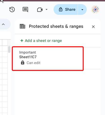
All of your previously created saved rules will be visible in a panel on the right side of the window when you select “Protect sheets and ranges.” As shown in the example that follows. Click on the rule that you want to unlock to unlock the row.
Step 4>
The stored rule will open in the following format when you click on it. However, to make changes, we must unlock our row and remove the protection. To do so, click the small “Bin” icon to remove the rule from the Protect sheets and ranges.

Step 5>
To unlock your row in Google Sheets, click the “Remove” button once a little pop-up confirms that you want to remove the protection. If you are certain that you want to remove this protection range, click the “Bin” button above.

How to freeze a row on Google Sheets?
In Google Sheets, rows that you freeze will remain visible when you scroll down. In the same way, columns that have been frozen will show up when you scroll to the right. This post will walk you through the process of freezing a row in Google Sheets if you need to do so.
Step 1>
In Google Sheets, you can freeze a row by dragging your mouse over it, as I’ve done in the example below.

Step 2>
Then, as shown in the screenshot below, select the “View” tab from the Google Sheets menu bar, which is situated right next to the File and Edit tab.

Step 3>
When you click on the “View” tab in the menu bar, a small drop-down menu with your built-in “Freeze” option will show up. To freeze a specific row or cell range on Google Sheets, click on it.

Step 4>
Upon selecting the “Freeze” option, a menu will expand and present you with many criteria to freeze any given range. Here, as indicated in the following image, choose the “Up to row()” option since we need to freeze a row.

Step 5>
The following GIF shows the result, Separating line shows that the cells have been frozen. Similarly, any row in Google Sheets can be frozen.

You may also like>>> How To Make A Stunning Chart In Google Sheets
Conclusion
One amazing feature that Google Sheets offers its users is the ability to lock a row on Google Sheets. The tutorial above teaches us how to lock a row in Google Sheets; hopefully, it will be useful. Thanks for learning with Office Chaser.